


-
林分结构是影响林分生长和发育的关键因素。林分结构对于林分生长以及收获量的影响已被许多研究所探讨[1-5]。在这些研究中,Bohn等[4]分析了305054株树进而发现林分的平均生长量不会随着物种多样性的增加而增加,而是与林分结构密切相关。林分结构受单木水平的生长差异影响,而单木水平的生长差异又由3个因素所决定:林分内的资源总量、林分能够获得的资源总量,以及林分对于这些资源的利用效率[5]。在这些影响森林生长的众多因素中,竞争起着重要的作用[6]。例如,伴随着林分的发展,大树会形成较大的树冠,使林分逐渐郁闭,在这种情形下,大树可以不成比例的获取光能,同时限制小树的生长[7]。
为了更直观地描述林分内林木个体的资源利用效率,Binkley等[7]提出了生长优势系数的概念来量化林分内部的生长动态。利用生长优势的概念,理论上可以将林分生长发育过程划分为4个阶段。在第一阶段,林分处于未郁闭状态,林木个体所获取的光能与其自身大小成比例,这与生长优势的0值相对应。伴随着大树树冠的生长,林分逐渐郁闭,限制了小树对于光能的获取,同时大树在不成比例地生长,生长优势的正值出现,对应于生长优势的第二阶段。到了第三阶段,生长优势又会重新接近于0值,因为林分内部经过一段时间的自伐后,竞争会逐渐减小,各株树的生长量又与自身的大小成比例。第四阶段对应于Oliver[8]提出的林分再生长阶段,在这个阶段,伴随着大树的老龄化,林分内优势地位会逐渐由大树向小树转移,即出现负的生长优势。然而,基于未经营管理林分观察到的生长优势变化规律与受经营管理的林分会截然不同,因为在林分经营管理过程中,林分内部的资源利用效率与林分结构可由人为调控。例如,下层间伐可以通过移除林分内低活力林木来提高保留木的资源利用效率,以及增加保留木的叶面积来提高林分收获量[9-10]。此外,不同树种的资源利用效率也不同。例如,一些耐荫树种的生长优势可能会低于非耐阴树种[11]。因此,需要更多的试验去验证生长优势在不同树种之间存在的普遍性,以及不同经营管理措施下生长优势的变化规律。
杉木是中国南方最重要的木材来源之一[12]。因其具有优良的木材性能,总种植面积达到了893万hm2,占人工造林面积的19.01%[13]。目前已经开展了许多关于杉木林密度效应的研究[14-18]。然而,对于杉木密度间伐林的资源利用效率的研究却鲜有人关注。在这项研究中,作者利用杉木密度间伐林来探究林分生长优势在间伐处理下的变化规律,旨在为杉木林栽培管理提供有效的管理策略以及丰富生长优势在不同树种之间发展的普遍性。因此,提出了以下假设:(1)生长优势会伴随着林龄的增加而增加,因为伴随着时间的推移,林分内部竞争会越来越强,大树的优势地位也越来越明显。(2)林分生长优势会伴随着累积间伐强度的增加而减少,因为累积间伐强度越大,林分内竞争越弱,林分内小树能获取的光能也更多,相对生长量也越大。(3)当不同初植密度林分间伐到相同保留密度时,高初植密度的生长优势会低于低初植密度样地,因为伴随着间伐的进行,高初植密度样地中的小树会比低初植密度样地的小树对于增加的光能反应更强烈。
-
试验样地设置在江西省分宜县大岗山实验局年珠林场青石湾,属于罗霞山脉北端的武功山支脉。地处于27°34′ N,114°33′ E,母岩为砂页岩,海拔450 m,气候为亚热带海洋季风气候,年平均降水量1656 mm,年平均温度16.8℃,年蒸发量1503 mm,土壤类型为黄壤。林下灌木有青冈栎(Cyclobalanopsis glauca (Thunberg.) Oersted.)、甜槠(Castanopsis eyrei (Champ. ex Benth.) Tutch.)、苦槠(Castanopsis sclerophylla (Lindl. et Paxton.) Schottky.)、木荷(Schima superba Gardn. (et Champ.))、红楠(Machilus thunbergii Sieb. (et Zucc.))、杜英(Elaeocarpus decipiens Hemsl.)、中华杜英(Elaeocarpus chinensis (Gardn. et Champ.) Hk. f. ex Benth.)等,林下草本植物有乌毛蕨(Blechnum orientale Linn.)、狗脊(Woodwardia japonica (L. F.) Sm.)、山姜(Alpinia japonica (Thunb.) Miq.)等。
-
试验林使用1年生苗木于1981年造林,采用完全随机区组设计,3次重复、5个处理。5个处理即为5种间距种植:A: 2 m × 3 m(1 667 株·hm−2),B: 2 m × 1.5 m(3 333 株·hm−2),C: 2 m × 1 m(5 000 株·hm−2),D: 1 m × 1.5 m(6 667 株·hm−2)以及E: 1 m × 1 m(10 000 株·hm−2)。共设置15个样地,每个样地20 m × 30 m。各样地的立地指数介于12~16之间。试验所需的数据,包括树高(H)与胸径(DBH),在1984年到1991年期间每年测量1次,从1992年开始到2006年,每2年测量1次。本研究中使用了1986年到2002年的数据。为了排除不等间隔期对生长分析的影响,研究中未使用1985年、1987年、1989年、1991年的数据。
在林分生长过程中,按照刘景芳等[14]编制的“杉木林分密度管理图”的密度管理线0.5为标准进行动态下层间伐。各密度处理的林分在不同的年龄进行了间伐(表1)。通常来说,林分在进行间伐的时候,林分密度会间伐到下一级密度水平。例如,E密度处理(10 000 株·hm−2)会间伐4次,首先会间伐到与D密度处理相同的密度水平(6 667 株·hm−2),而后间伐到C密度处理(5 000 株·hm−2)相同的密度水平,再间伐到B密度处理(3 333 株·hm−2)的密度水平,最后间伐到与A密度处理(1 667 株·hm−2)相同的密度水平,其他初植密度处理以此类推。到22年生时,除了第一区组的B1、D1、E1小区以外,其他的12个小区的存活株数均处于1 667 株·hm−2左右。各密度样地基本特征见表2。
表 1 样地每公顷保留株数变化情况
Table 1. The development of number of living trees per hectare
样地 Plot 林龄 Age/a 6 8 9 10 11 12 14 16 18 20 22 A1 1 634 1 634 1 600 1 584 1 584 1 584 1 584 1 584 1 584 1 584 1 550 A2 1 634 1 617 1 600 1 600 1 584 1 584 1 584 1 584 1 584 1 584 1 534 A3 1 617 1 617 1 584 1 584 1 584 1 584 1 567 1 567 1 534 1 534 1 500 B1 3 284 3 251 3 217 3 167 3 167 3 151 3 084 2 884 2 751 2 751 2 617 B2 3 234 3 217 3 217 3 217 3 201 3 184 3 151 3 151 1 550 1 550 1 550 B3 3 217 3 217 3 151 3 134 3 134 3 134 3 051 2 934 1 684 1 684 1 684 C1 4 751 4 668 4 618 4 501 4 501 4 401 3 334 3 334 1 717 1 667 1 667 C2 4 801 4 801 4 718 4 718 4 718 3 334 3 301 1 667 1 617 1 617 1 600 C3 4 901 4 851 4 818 4 718 4 634 3 334 3 317 1 667 1 667 1 667 1 667 D1 6 385 6 251 6 101 5 918 5 918 5 568 5 468 5 001 3 351 3 351 3 351 D2 6 385 6 235 5 935 5 001 5 001 3 217 3 217 1 667 1 667 1 667 1 650 D3 6 518 6 468 6 301 4 951 4 951 3 351 3 334 1 667 1 667 1 650 1 650 E1 9 585 9 369 6 668 6 668 6 668 4 984 4 951 3 317 3 301 3 301 3 267 E2 9 369 9 269 6 668 6 635 4 951 3 301 3 301 3 301 1 800 1 800 1 767 E3 9 685 9 602 6 735 6 735 5 068 3 317 3 301 1 667 1 617 1 617 1 617 注:红色标注的数字代表样地在上一个观测年进行了间伐。
Note: The number in redrepresents the plot was thinned in last observation.表 2 杉木林分及林木各变量统计值
Table 2. Summary statistics of stand and tree variables of Chinese fir plantations
初值密度
Initial planting density林分平均直径
Stand mean diameter/cm优势木平均高
Dominant height/m林分断面积
Stand basal area/(m2·hm−2)林分蓄积量
Stand volume/(m3·hm−2)平均值
Mean标准差
SD.平均值
Mean标准差
SD.平均值
Mean标准差
SD.平均值
Mean标准差
SD.2 m × 3 m 14.68 4.89 13.33 4.85 31.09 15.74 210.33 143.49 2 m × 1.5 m 12.42 4.27 13.73 3.79 33.41 15.43 219.99 126.99 2 m × 1 m 12.58 4.92 13.45 3.69 34.87 12.07 210.01 110.47 1 m × 1.5 m 11.40 5.27 12.20 3.82 33.68 13.35 192.79 117.45 1 m × 1 m 10.88 5.00 11.47 3.80 31.79 10.87 167.25 94.63 -
根据Zhang等[19]提供的生物量模型估算杉木树干生物量。具体模型如下:
$ W = {\rm{ }}{{\rm{e}}^{ - 2.830\;5}}{\left( {{D^2} \times H} \right)^{0.806\;7}} $
其中W代表树干生物量,D代表胸径,H代表树高。
根据West[20]提出的生长优势的计算方法,其计算公式如下:
$ GD=1-\sum _{i=1}^{n}({x}_{i}-{x}_{i-1})({y}_{i}+{y}_{i-1}) $
在模型中,x代表累积树干生物量百分比,分母为林分总生物量,y代表累积树干生物量增量百分比,分母为林分总生物量增量,n代表样地内立木株数。生长优势的正值代表大树对于林分生长的贡献量要大于其对于林分生物量的贡献量。生长优势的负值代表大树对于林分生长的贡献量要小于其对于林分生物量的贡献量。生长优势的0值代表林分内所有林木对于林分生长的贡献量等于其对于林分生物量的贡献量。
为了探究累积间伐强度、林龄以及保留株数密度对林分水平生长优势的影响,以生长优势作为响应变量,以累积间伐强度、保留株数密度以及林龄作为自变量,构建线性混合效应模型。累积间伐强度是指第一个观测年的样地株数与间伐后的保留株数密度之差与第一个观测年的样地株数的比值。模型的随机效应为区组,重复效应为林龄。模型分析利用R软件中的软件包“nlme”完成[21]。
因为生长差异分析对比需以立地质量相同为前提条件,所以,针对不同立地质量的样地,分别制作了保留株数密度与累积间伐强度对于生长优势影响的三维图。
-
最终的生长优势模型包括主效应累积间伐强度、林龄、保留株数密度以及交互项林龄 × 累积间伐强度、累积间伐强度 × 保留密度。模型数学表达式为:
$ \begin{split} &\qquad GD=0.042N+1.154T+0.009A-0.016\left(A\times T\right)-\\ &0.115\left(N\times T\right)-0.42 \end{split}$
式中,GD代表林分生长优势,N代表每公顷保留密度,T代表累积间伐强度,A代表林龄,A × T代表林龄与累积间伐强度的交互作用,N × T代表保留密度与累积间伐强度的交互作用。
模型拟合的结果如表3所示,生长优势伴随累积间伐强度、林龄以及保留密度的增加而增加(P < 0.05),表明林分内大树的相对生长量随着累积间伐强度、林龄以及保留密度的增加而增加。林龄与累积间伐强度的交互项表明,生长优势伴随着林龄的变化在不同的累积间伐强度之间是有差异的。保留密度与累积间伐强度的交互项表明,不同累积间伐强度下,不同保留密度样地的生长优势是有差异的。
表 3 生长优势的混合效应模型结果
Table 3. The results of mixed effect models of growth dominance
项目 Items 模型 Model 参数 Parameter P值 P-value 保留密度 Residual density 0.042 0.000 7 累积间伐强度 Accumulate thinning intensity 1.154 0.008 9 林龄 Age 0.009 < 0.000 1 林龄 × 累积间伐强度 Age × Accumulate thinning intensity −0.016 0.003 5 保留密度 × 累积间伐强度 Residual density × Accumulate thinning intensity −0.115 0.018 2 注:参数是指混合效应模型中各自变量的参数。P值为混合效应模型F检验的P值。累积间伐强度为第一个观测年的样地存活株数与间伐后的保留株数密度之差与第一个观测年的样地存活株数的比值。保留密度为林分中每公顷存活株数。年龄为林龄。
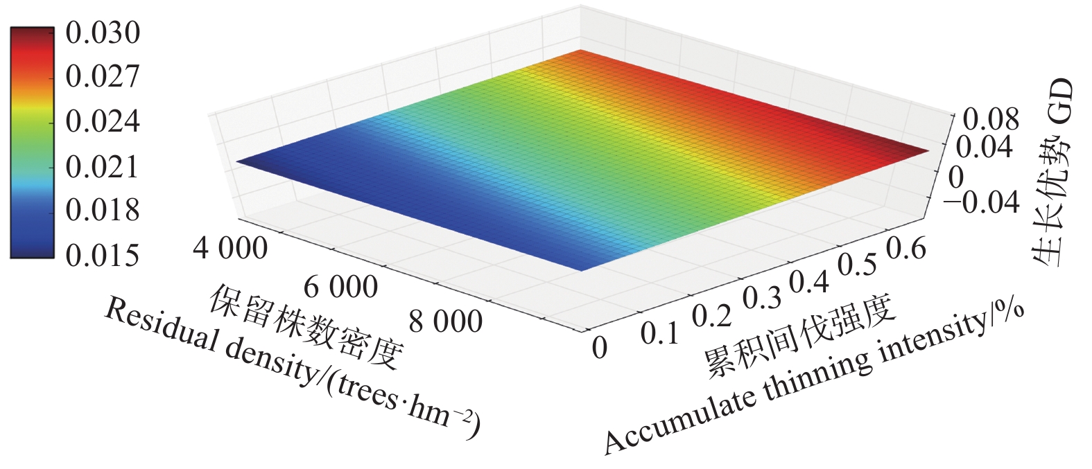
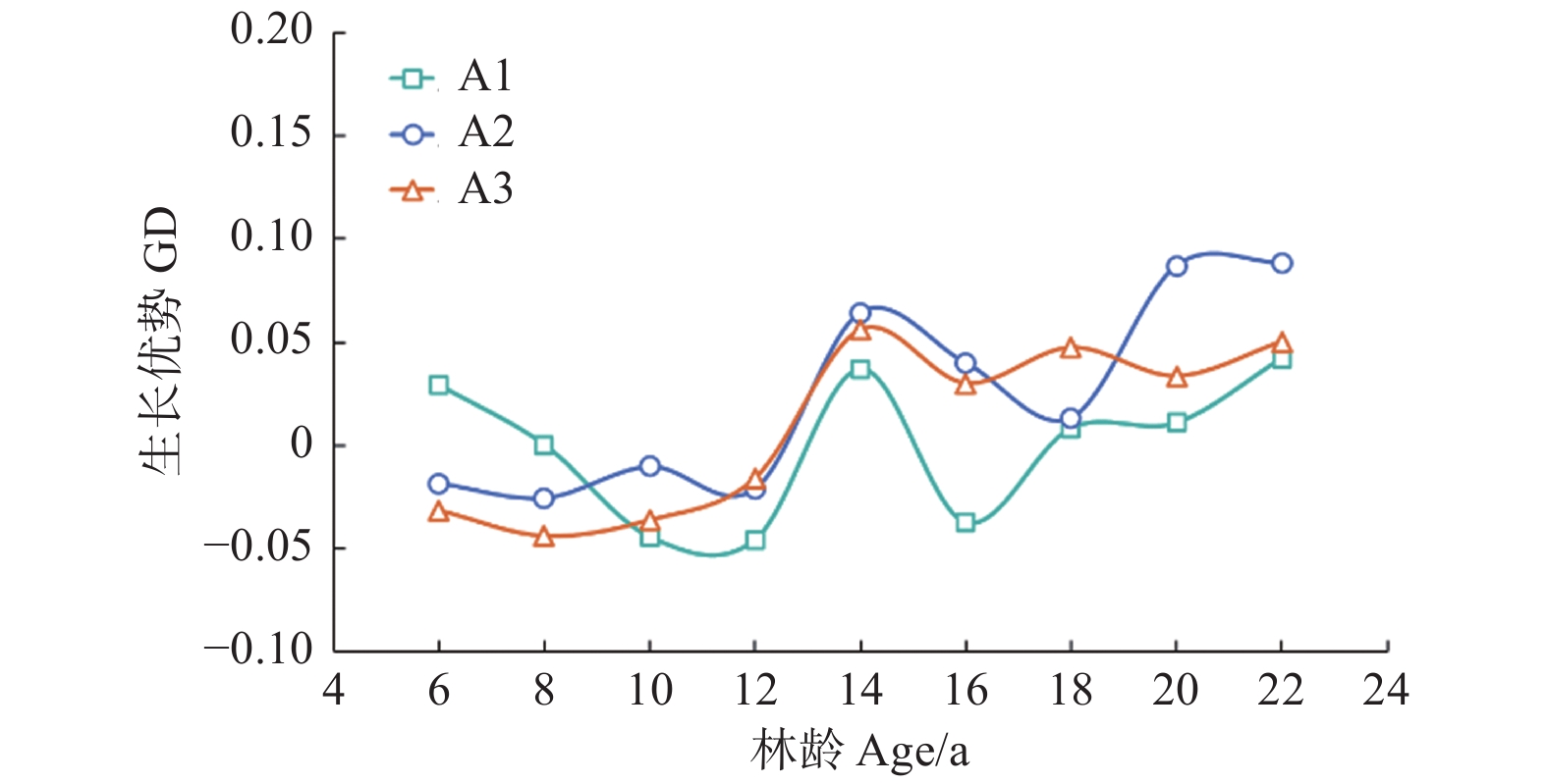
Note:Parameter refers to the parameter of the independent variable in the mixed effect model. The P-values refers to the P-values of F-tests for growth dominance model. Accumulate thinning intensity refers to the ratio of the difference between the number of living trees of the first observation and the residual density caused by thinning to the number of living trees of the first observation. Residual density refers to the number of living trees per ha in stands. Age refers to the stand age.对于未间伐林分(A密度:1 667 株·hm−2)的生长优势变化规律而言,所有样地的生长优势伴随着年龄的增加都呈上升趋势。生长优势的负值大多出现在前期(林龄 < 14年生)(图1)。对于同一立地指数和相同保留密度下,不同累积间伐强度的生长优势变化规律而言,林分水平的生长优势均伴随着累积间伐强度的增加而增加(图2~4)。
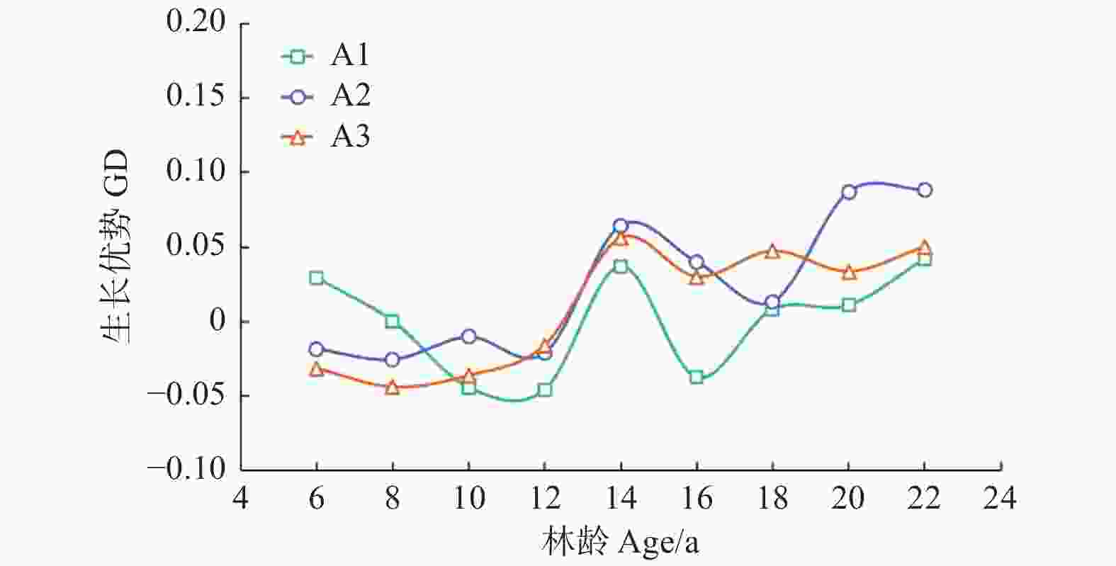
图 1 未间伐样地(A密度)生长优势伴随林龄的变化规律
Figure 1. The growth dominance of unthinned stands develop with stand age
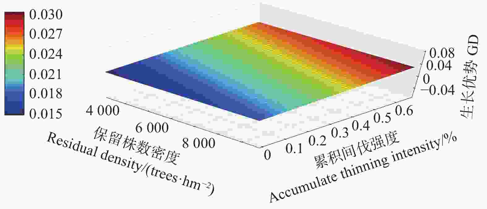
图 2 生长优势伴随保留株数密度以及累积间伐强度的变化规律(12指数级)
Figure 2. The growth dominance develop with residual density and accumulate thinning intensity (12 index)
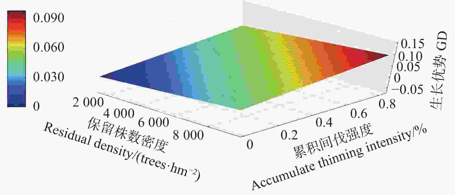
图 3 生长优势伴随保留株数密度以及累积间伐强度的变化规律(14指数级)
Figure 3. The growth dominance develop with residual density and accumulate thinning intensity (14 index)

图 4 生长优势伴随保留株数密度以及累积间伐强度的变化规律(16指数级)
Figure 4. The growth dominance develop with residual density and accumulate thinning intensity (16 index)
-
一个普遍被各研究者所认同的观点是,伴随林分的发展,生长优势会呈现出逐渐上升的趋势,即林分一定会出现生长优势模型的第二阶段[22-23]。本研究结果与我们的假设(1)一致:生长优势伴随着林龄的增加而增加,并验证了Binkley等[7]提出的生长优势假说的第二阶段。这与Soares等[5]对桉树在间伐处理下的生长优势与基尼系数变化规律的研究中所得结果一致,其认为在间伐前后,生长优势会随着林龄的增加而出现上升的趋势。同样,Bradford等[24]与Moreau等[10]对生长优势在间伐作用下的变化规律研究也验证了这一点。
关于负生长优势的研究,不同树种,其研究结果也不同。例如,Binkley等[7]对多个树种生长优势的变化规律进行了研究,发现除杨树(Populus tremuloides Linn.)外,其他树种如云杉(Picea engelmannii Parry ex Engelm.)、西黄松(Pinus ponderosa Douglas ex C. Lawson.)、冷杉(Abies lasiocarpa (Hook.) Nutt.)均观测到了持续的负生长优势。Doi等[25]利用桉树(Eucalyptus saligna (Smith.))验证了生长优势的第四阶段,然而结果中也未出现负的生长优势。在本研究中,负生长优势并未在最后一个观测年(22年生)出现。我们认为这种情况是由于树种生理结构的差异或者林分林龄相对较小的原因所导致。对于不同树种具有不同的生长优势变化规律的假设已在其他研究中得到了验证[10,26]。对于林龄而言,在最后的观测年,试验林林龄为22年生,相对于其他树种研究中持续出现负生长优势的林龄来说还很年轻[7]。
此外,在本研究中,负生长优势意外的出现在林分发展的初始阶段(林龄 < 14年生),这与生长优势模型第一阶段向第二阶段由0向正值变化的假设不相符。我们认为这是因为样地初植密度较稀疏而导致林分持续未郁闭所造成的。这也与Fernández Tschieder等[26]利用西黄松探究林内不同大小树木生长效能的差异所观察到的结果一致,其结果中显示,在林内空间较开阔的情况下,大树与小树的生长效能无差异。所以,林分初始阶段的生长优势并非都由0值开始,也可能是负值。
-
通常来说,下层间伐不仅可以重新分配立地资源,减少林木死亡损失,而且还可以增加保留木的活力,降低林分内部竞争,从而促进保留木中小树对光能的获取[27]。这在许多的研究中得到了验证[22-23]。然而,我们的结果与假设(2)不一致,生长优势随累积间伐强度的增加而呈上升趋势,在排除小树出现显著生长,生物量超过大树的情况下,这说明在间伐后林分内优势地位没有向小树转移,间伐反而促进了大树的生长。
这种情况可以用保留木中大树对于间伐的反应以及树种不同的生理结构来解释。杉木作为一种针叶树,其对于光能的需求量要少于阔叶树。这在Pothier [11]对不同耐荫树种生长优势的变化规律研究中也得到了验证。所以推测,杉木林分内部竞争主要来自于林分林木对于地下资源的竞争,而不是光能的竞争。当林分内低活力林木被移除时,林分内可用资源的增加促使大树更进一步不成比例地获取资源。这些结果突出了生长优势作为评价杉木林营林处理的一种工具的潜力。因为间伐的一个重要目的是就是为了减少竞争,以便有限的资源可以更均匀地分配在保留木中。
-
一般来说,当不同初植密度林分间伐到相同保留密度后,林分生长优势会随初植密度的增加而减小,因为高初植密度林分内大树在间伐前已经不成比例地获取了足够的资源,通过移除林分内低活力林木可能不会再增加他们的资源获取效率,进而引起大树对间伐积极的生长反应[28-30]。然而,与假设(3)相反,不同初植密度的林分间伐到相同的保留密度后,各样地生长优势随着累积间伐强度的增加而增加。这可能是因为林分内树木在间伐前为了获取资源而经历了激烈的相互竞争的原因。这与Lemire等[23]利用生长优势作为评价措施去评价选择间伐的效果所得结果一致,其发现一些间伐前生长缓慢的大树在选择间伐后相对生长量出现了增加。此外,也有一些研究表明,通过间伐来减少林分内部竞争可能会增加大树的资源利用效率[31-33]。所以,我们认为当不同的杉木林初植密度样地间伐到相同密度时,累积间伐强度越强,大树的资源利用效率也越高。
-
本研究利用杉木密度间伐林为期16年的连续调查数据,探究了不同初值密度林分的生长优势在间伐处理下的变化规律。结果表明,未间伐样地的生长优势伴随林龄的增加呈上升趋势;间伐样地的生长优势随累积间伐强度、林龄以及保留株数密度的增加而增加;当不同初值密度的样地间伐到相同保留密度后,高初植密度样地的生长优势要高于低初植密度样地。这为杉木林营林提供了宝贵的密度调控建议,当造林目的是收获大径材时,我们可以进行低密度种植,低密度管理,因为间伐到目标密度后,相对于高初植密度样地,低初植密度样地的生长优势更低,各株树的生长比较均衡,所收获的大径材比例比较高。鉴于下层间伐后,林分的直径分布近似于“钟型”,相对较低的生长优势意味着会极大促进林分内主体即中小树木的生长。如果市面上既需要中小径材,又需要大径材,可以进行高密度种植,低密度管理,因为在间伐收获小树的同时,伴随着累积间伐强度的增强还可以促进林分内大树的生长。
杉木人工林不同密度间伐林分生长优势的变化规律分析
Variation of Growth Dominance in Thinned Chinese Fir Stands with Different Planting Densities
-
摘要:
目的 利用杉木密度间伐林探究林分生长优势在间伐处理下的变化规律,为杉木林栽培管理提供有效的管理策略。 方法 以江西省分宜年珠林场青石湾杉木密度间伐林为研究对象,用线性混合效应模型分析了生长优势与林龄、累积间伐强度、保留株数密度以及这些变量相互作用的关系。 结果 在间伐前后,生长优势伴随着累积间伐强度、林龄以及保留株数密度的增加而增加。生长优势的负值未在最后的观测年出现。同一保留株数密度下,生长优势随累积间伐强度的增加而增加。 结论 低密度种植,低密度管理,使得生长优势更趋近于0,有利于林木均衡生长,提高大径材产量。高密度种植,低密度管理不仅在间伐收获小树的同时,伴随着累积间伐强度的增强,生长优势增加,促进林分内大树的生长,从而收获大径材。 Abstract:Objective The thinned Chinese fir (Cunninghamia lanceolata) stands with different planting densities were used to explore the variation of growth dominance under different thinning treatments, so as to provide management strategies for cultivation and management of Chinese fir. Method The data for this study were sampled from Chinese fir plantation in Nianzhu Forest Farm, Fenxi city, Jiangxi Province. The linear mixed effect model was used to illustrate the growth dominance in relation to age, accumulated thinning intensity, living number of trees per hectare and the interaction of these variables. Result The growth dominance increased with accumulated thinning intensity, age, and living number of trees per hectare before or after the thinning. The negative value of growth dominance was not observed during the last observation. When the stands had the same living number of trees per hectare, the growth dominance increased with accumulated thinning intensity. Conclusion The sparse planting density and sparse density management make the growth dominance closer to the value 0, which is beneficial for balanced growth of all sized trees, and increasing the yield of larger trees. The dense planting density and sparse density management can not only harvest smaller trees, but also increase the growth dominance and promote the growth of larger trees with the increase of accumulated thinning intensity, as a result of harvesting the large size trees. -
Key words:
- growth dominance
- / thinning
- / planting density
- / competition
- / Cunninghamia lanceolata
-
图 1 未间伐样地(A密度)生长优势伴随林龄的变化规律
Figure 1. The growth dominance of unthinned stands develop with stand age
图 2 生长优势伴随保留株数密度以及累积间伐强度的变化规律(12指数级)
Figure 2. The growth dominance develop with residual density and accumulate thinning intensity (12 index)
图 3 生长优势伴随保留株数密度以及累积间伐强度的变化规律(14指数级)
Figure 3. The growth dominance develop with residual density and accumulate thinning intensity (14 index)
图 4 生长优势伴随保留株数密度以及累积间伐强度的变化规律(16指数级)
Figure 4. The growth dominance develop with residual density and accumulate thinning intensity (16 index)
表 1 样地每公顷保留株数变化情况
Table 1. The development of number of living trees per hectare
样地 Plot 林龄 Age/a 6 8 9 10 11 12 14 16 18 20 22 A1 1 634 1 634 1 600 1 584 1 584 1 584 1 584 1 584 1 584 1 584 1 550 A2 1 634 1 617 1 600 1 600 1 584 1 584 1 584 1 584 1 584 1 584 1 534 A3 1 617 1 617 1 584 1 584 1 584 1 584 1 567 1 567 1 534 1 534 1 500 B1 3 284 3 251 3 217 3 167 3 167 3 151 3 084 2 884 2 751 2 751 2 617 B2 3 234 3 217 3 217 3 217 3 201 3 184 3 151 3 151 1 550 1 550 1 550 B3 3 217 3 217 3 151 3 134 3 134 3 134 3 051 2 934 1 684 1 684 1 684 C1 4 751 4 668 4 618 4 501 4 501 4 401 3 334 3 334 1 717 1 667 1 667 C2 4 801 4 801 4 718 4 718 4 718 3 334 3 301 1 667 1 617 1 617 1 600 C3 4 901 4 851 4 818 4 718 4 634 3 334 3 317 1 667 1 667 1 667 1 667 D1 6 385 6 251 6 101 5 918 5 918 5 568 5 468 5 001 3 351 3 351 3 351 D2 6 385 6 235 5 935 5 001 5 001 3 217 3 217 1 667 1 667 1 667 1 650 D3 6 518 6 468 6 301 4 951 4 951 3 351 3 334 1 667 1 667 1 650 1 650 E1 9 585 9 369 6 668 6 668 6 668 4 984 4 951 3 317 3 301 3 301 3 267 E2 9 369 9 269 6 668 6 635 4 951 3 301 3 301 3 301 1 800 1 800 1 767 E3 9 685 9 602 6 735 6 735 5 068 3 317 3 301 1 667 1 617 1 617 1 617 注:红色标注的数字代表样地在上一个观测年进行了间伐。
Note: The number in redrepresents the plot was thinned in last observation. 下载: 导出CSV
表 2 杉木林分及林木各变量统计值
Table 2. Summary statistics of stand and tree variables of Chinese fir plantations
初值密度
Initial planting density林分平均直径
Stand mean diameter/cm优势木平均高
Dominant height/m林分断面积
Stand basal area/(m2·hm−2)林分蓄积量
Stand volume/(m3·hm−2)平均值
Mean标准差
SD.平均值
Mean标准差
SD.平均值
Mean标准差
SD.平均值
Mean标准差
SD.2 m × 3 m 14.68 4.89 13.33 4.85 31.09 15.74 210.33 143.49 2 m × 1.5 m 12.42 4.27 13.73 3.79 33.41 15.43 219.99 126.99 2 m × 1 m 12.58 4.92 13.45 3.69 34.87 12.07 210.01 110.47 1 m × 1.5 m 11.40 5.27 12.20 3.82 33.68 13.35 192.79 117.45 1 m × 1 m 10.88 5.00 11.47 3.80 31.79 10.87 167.25 94.63
下载: 导出CSV
表 3 生长优势的混合效应模型结果
Table 3. The results of mixed effect models of growth dominance
项目 Items 模型 Model 参数 Parameter P值 P-value 保留密度 Residual density 0.042 0.000 7 累积间伐强度 Accumulate thinning intensity 1.154 0.008 9 林龄 Age 0.009 < 0.000 1 林龄 × 累积间伐强度 Age × Accumulate thinning intensity −0.016 0.003 5 保留密度 × 累积间伐强度 Residual density × Accumulate thinning intensity −0.115 0.018 2 注:参数是指混合效应模型中各自变量的参数。P值为混合效应模型F检验的P值。累积间伐强度为第一个观测年的样地存活株数与间伐后的保留株数密度之差与第一个观测年的样地存活株数的比值。保留密度为林分中每公顷存活株数。年龄为林龄。
Note:Parameter refers to the parameter of the independent variable in the mixed effect model. The P-values refers to the P-values of F-tests for growth dominance model. Accumulate thinning intensity refers to the ratio of the difference between the number of living trees of the first observation and the residual density caused by thinning to the number of living trees of the first observation. Residual density refers to the number of living trees per ha in stands. Age refers to the stand age.
下载: 导出CSV
-
[1] 袁秀锦, 肖文发, 潘 磊, 等. 马尾松林分结构对枯落物层和土壤层水文效应的影响[J]. 林业科学研究, 2020, 33(4):26-34. [2] 高成杰, 唐国勇, 刘方炎, 等. 林分结构调整对云南松次生林生长和土壤性质的影响[J]. 林业科学研究, 2017, 30(5):841-847. [3] Binkley D, Stape J L, Ryan M G, et al. Age-related decline in forest ecosystem growth: an individual-tree, stand-structure hypothesis[J]. Ecosystems, 2002, 5: 58-67. doi: 10.1007/s10021-001-0055-7 [4] Bohn F J, Huth A. The importance of forest structure to biodiversity-productivity relationships[J]. R Soc Open Sci, 2017, 4(1): 160521. doi: 10.1098/rsos.160521 [5] Soares A A V, Leite H G, Cruz J P, et al. Development of stand structural heterogeneity and growth dominance in thinned Eucalyptus stands in Brazil[J]. For Ecol Manage, 2017, 384: 339-346. doi: 10.1016/j.foreco.2016.11.010 [6] Wang W, Chen X, Zeng W, et al. Development of a mixed-effects individual-tree basal area increment model for oaks (Quercus spp.) considering forest structural diversity[J]. Forests, 2019, 10(6): 474. doi: 10.3390/f10060474 [7] Binkley D, Kashian D M, Boyden S, et al. Patterns of growth dominance in forests of the Rocky Mountains, USA[J]. For Ecol Manage, 2006, 236(2-3): 193-201. doi: 10.1016/j.foreco.2006.09.001 [8] Oliver C D. Forest development in North America following major disturbances[J]. For Ecol Manage, 1981, 3(3): 153-168. [9] Long J N, Dean T J, Roberts S D. Linkages between silviculture and ecology: examination of several important conceptual models[J]. For Ecol Manage, 2004, 200(1-3): 249-261. doi: 10.1016/j.foreco.2004.07.005 [10] Moreau G, Auty D, Pothier D, et al. Long-term tree and stand growth dynamics after thinning of various intensities in a temperate mixed forest[J]. For Ecol Manage, 2020, 473: 0378-1127. [11] Pothier D. Relationships between patterns of stand growth dominance and tree competition mode for species of various shade tolerances[J]. For Ecol Manage, 2017, 406: 155-162. doi: 10.1016/j.foreco.2017.09.066 [12] 吴中伦. 杉木[M]. 北京: 中国林业出版社, 1984. [13] Zhang X, Cao Q, Wang H, et al. Projecting stand survival and basal area based on a self-thinning model for Chinese fir plantations[J]. For Sci, 2020, 66(3): 361-370. doi: 10.1093/forsci/fxz086 [14] 刘景芳, 童书振. 编制杉木林分密度管理图研究报告[J]. 林业科学, 1980, 16(4):241-251. [15] 贾亚运, 何宗明, 周丽丽, 等. 造林密度对杉木幼林生长及空间利用的影响[J]. 生态学杂志, 2016, 35(5):1177-1181. [16] 童书振, 盛炜彤, 张建国. 杉木林分密度效应研究[J]. 林业科学研究, 2002, 15(1):66-75. doi: 10.3321/j.issn:1001-1498.2002.01.011 [17] 相聪伟, 张建国, 段爱国, 等. 杉木林分蓄积生长的密度及立地效应[J]. 林业科学研究, 2014, 27(6):801-808. [18] 相聪伟, 张建国, 段爱国, 等. 杉木人工林材种结构的立地及密度效应研究[J]. 林业科学研究, 2015, 28(5):654-659. doi: 10.3969/j.issn.1001-1498.2015.05.008 [19] Zhang X, Duan A, Zhang J, et al. Tree biomass estimation of Chinese fir (Cunninghamia lanceolata) based on bayesian method[J]. PLoS ONE, 2013, 8(11): e79868. doi: 10.1371/journal.pone.0079868 [20] West P W. Calculation of a growth dominance statistic for forest stands[J]. For Sci, 2014, 60(6): 1021-1023. doi: 10.5849/forsci.13-186 [21] Pinheiro J, Bates D, DebRoy S, et al. nlme: Linear and NonlinearMixed Effects Models[M]. New York, USA: R package version 3.1-121, 2015, pp: 121. [22] Forrester D I. Linking forest growth with stand structure: Tree size inequality, tree growth or resource partitioning and the asymmetry of competition[J]. For Ecol Manage, 2019, 447: 139-157. doi: 10.1016/j.foreco.2019.05.053 [23] Lemire C, Bédard S, Guillemette F, et al. Changes in growth dominance after partial cuts in even- and uneven-aged northern hardwood stands[J]. For Ecol Manage, 2020, 466: 118115. doi: 10.1016/j.foreco.2020.118115 [24] Bradford J B, D'Amato A W, Palik B J, et al. A new method for evaluating forest thinning: growth dominance in managed pinus resinosa stands[J]. Can J For Res, 2010, 40(5): 843-849. doi: 10.1139/X10-039 [25] Doi B T, Binkley D, José LuizStape. Does reverse growth dominance develop in old plantations of Eucalyptus saligna[J]. For Ecol Manage, 2010, 259(9): 1815-1818. doi: 10.1016/j.foreco.2009.05.031 [26] Fernández T E, Gyenge J. Testing Binkley 's hypothesis about the interaction of individual tree water use efficiency and growth efficiency with dominance patterns in open and close canopy stands[J]. For Ecol Manage, 2009, 257(8): 1859-1865. doi: 10.1016/j.foreco.2009.02.012 [27] Bédard S, Majcen Z. Growth following single-tree selection cutting in Quebec northern hardwoods[J]. For Chron, 2003, 79(5): 898-905. [28] Cameron A D. Importance of early selective thinning in the development of long-term stand stability and improved log quality: a review[J]. Forestry, 2002, 75(1): 25-35. doi: 10.1093/forestry/75.1.25 [29] Singer M T, Lorimer C G. Crown release as a potential old-growth restoration approach in northern hardwoods[J]. Can J For Res, 1997, 27(8): 1222-1232. doi: 10.1139/x97-071 [30] Boyden S, Montgomery R, Reich P B, et al. Seeing the forest for the heterogeneous trees: stand-scale resource distributions emerge from tree-scale structure[J]. Ecol Appl, 2012, 22: 1578-1588. [31] Jones T A, Thomas S C. Leaf-level acclimation to gap creation in mature Acer saccharum trees[J]. Tree Physiol, 2007, 27(2): 281-290. doi: 10.1093/treephys/27.2.281 [32] Wyckoff P H, Clark J S. Tree growth prediction using size and exposed crown area[J]. Can J For Res, 2005, 35(1): 13-20. doi: 10.1139/x04-142 [33] Hartmann H, Beaudet M, Mazerolle M J, et al. Sugar maple (Acer saccharum Marsh.) growth is influenced by close conspecifics and skid trail proximity following selection harvest[J]. For Ecol Manage, 2009, 258(5): 823-831. doi: 10.1016/j.foreco.2009.05.028 -

 点击查看大图
计量
- 文章访问数: 5681
- HTML全文浏览量: 3400
- PDF下载量: 136
- 被引次数: 0


